JSONB vs Normalised Tables: The Question Isn't "Which Is Better"

Series: Building Backarch, engineering decisions from building backarch.com

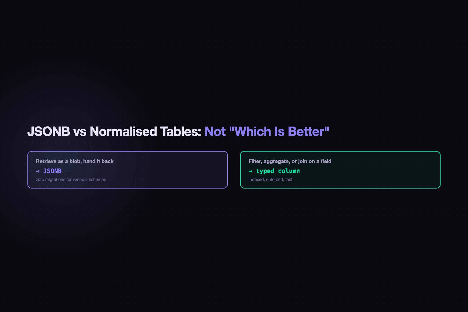
"Should I use JSONB or a normalised table?" is the wrong question. The right question is: how do you query this data?

JSONB and typed columns aren't competing strategies. They're tools for different access patterns. Choosing between them requires knowing what queries you'll actually run, not which one feels more principled.

The normalization temptation has a sharp edge

Imagine you're building a canvas tool with 75 component types: API gateways, Lambda functions, Postgres instances, Kafka brokers, GPU nodes, vector databases. Each has different config fields. A Lambda needs memory_mb and runtime. A Postgres instance needs instance_type, region, and storage_gb. A Kafka needs partition_count, replication_factor, and retention_hours.

The normalised path looks responsible: one row per node, config in typed columns. You write the first migration. Two weeks later, product adds a new node type. Another migration. Then another. You now have a migration per node type, each adding nullable columns that almost no row will ever use.

The EAV alternative, (entity_id, attribute_name, attribute_value), trades the migration problem for the query problem. You can't enforce types. You can't index efficiently. Reconstructing a single entity requires joining five rows. Both instincts fail because neither matches the actual shape of the data.

How React Flow made the decision obvious

When you build on React Flow, the framework hands you a format. A node looks like this:

{
  "id": "node-abc",
  "type": "lambda",
  "position": { "x": 320, "y": 180 },
  "data": {
    "name": "Auth Handler",
    "config": { "memory_mb": "256", "runtime": "nodejs20.x" },
    "pricing": { "label": "$5.00/mo", "monthly": 5.0 }
  }
}

In Backarch, diagram_versions.nodes is a JSONB array of exactly this structure. edges is a JSONB array of React Flow edge objects. Both are stored as-is, zero transformation. When you save, you pass the array straight through. When you load, you hand it back.

Adding a new node type, a timescaledb node with a retention_days config field, costs zero migrations. Add a row to the service_catalog table via seed script. The JSONB schema didn't move.

The queries that matter for canvas nodes are:

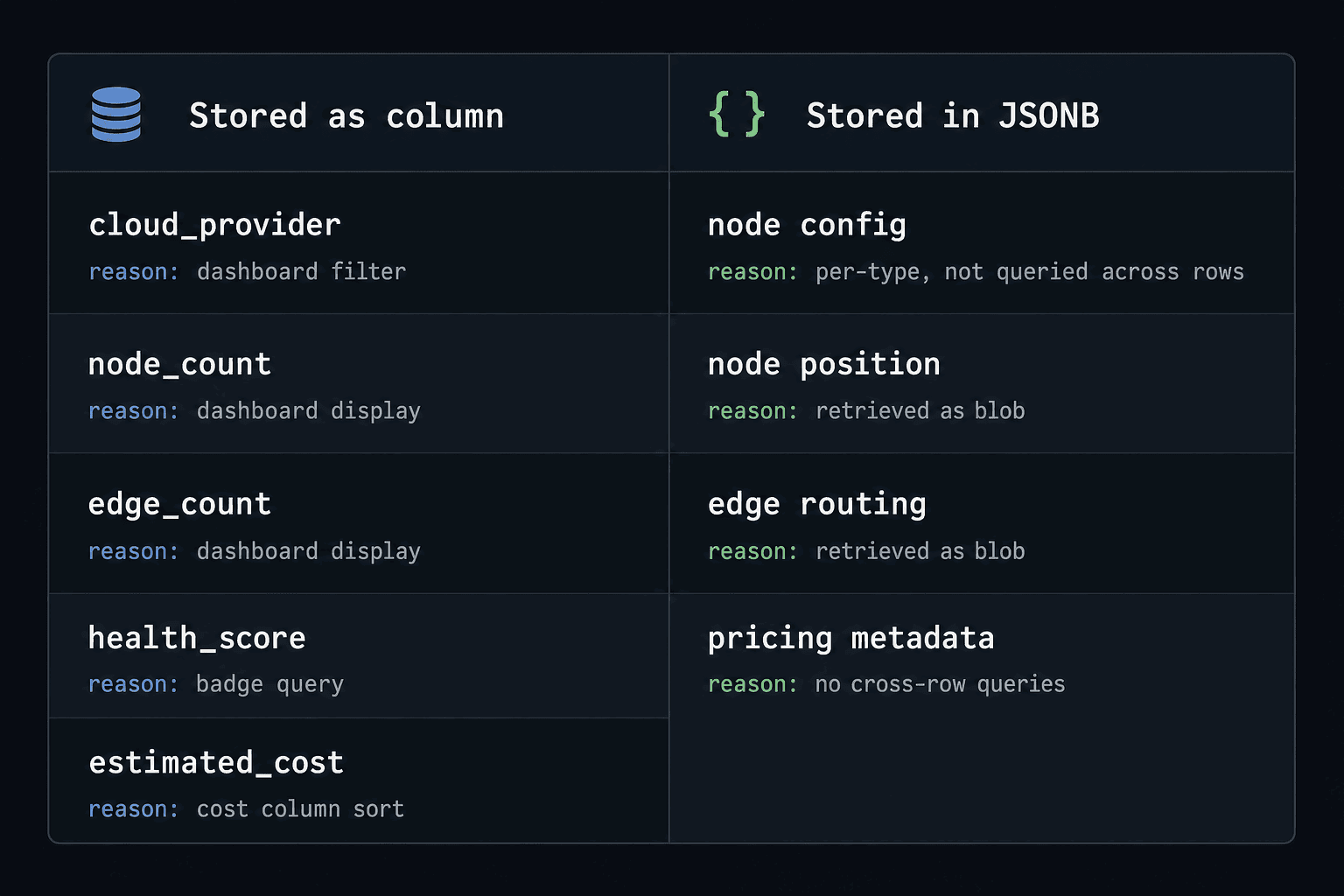
• "Give me all nodes for this diagram." → Single-row fetch on diagram_id. No index into JSONB needed.
• "How many nodes does this diagram have?" → Stored as node_count integer column, computed at save time.
• "What's the cloud provider of this diagram?" → Stored as cloud_provider text column, computed at save time.

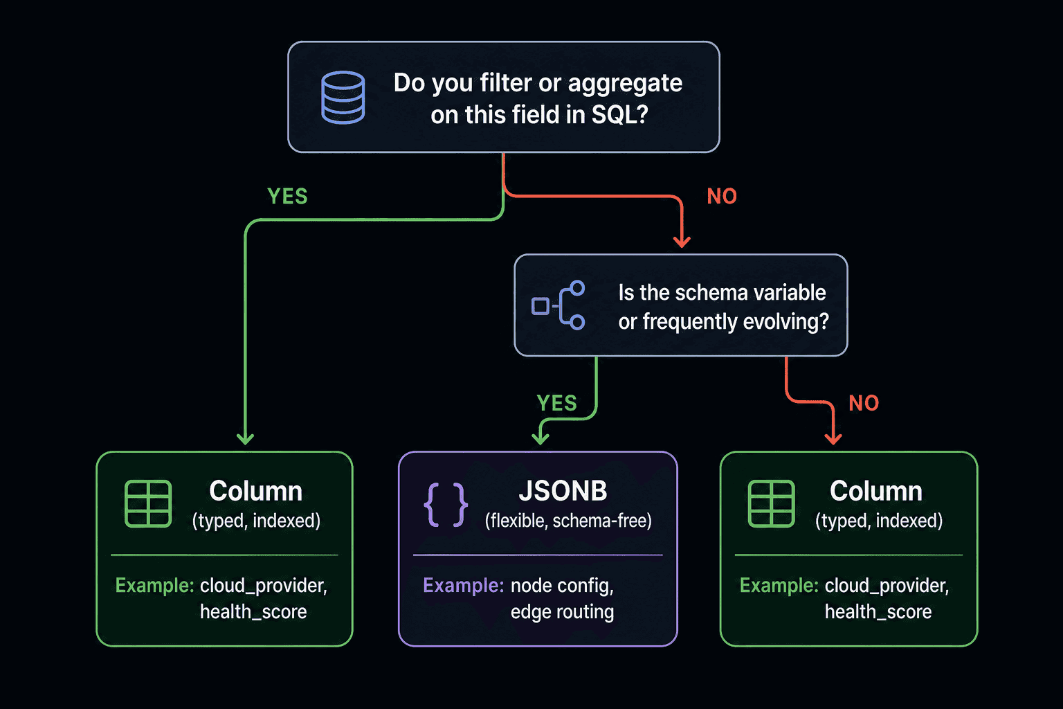
None of the real queries require filtering on JSONB fields across rows. JSONB wins.

When to break fields out into columns

The rule: if you filter or aggregate on a field in more than roughly 80% of queries, it belongs in a column. The dashboard list view filters diagrams by cloud provider. That's a frequent query on a bounded enum value. It's a stored column.

# diagram_versions: computed fields stored as typed columns
node_count:      Mapped[int]           # dashboard: "X nodes"
edge_count:      Mapped[int]           # same
cloud_provider:  Mapped[str | None]    # dashboard filter: "AWS" | "GCP" | "Azure"
health_score:    Mapped[float | None]  # dashboard badge
estimated_cost:  Mapped[Decimal | None]# dashboard cost column

These are derived from the JSONB at save time and written as first-class columns. The JSONB is the source of truth for the canvas state. The columns are the materialised view for the dashboard.

config.instance_type inside a node? Nobody queries across all diagrams for "all Postgres nodes running on db.t3.micro." That lives in JSONB.

What you're trading away with JSONB

JSONB is not free. Know what you're giving up:

You can't add a NOT NULL constraint on data.name. If a client sends a malformed node, PostgreSQL stores it without complaint. Schema validation moves entirely to Pydantic. The application layer enforces what the database layer can't. This is a real tradeoff: bugs that a typed schema would catch at insert time become silent data quality issues you only discover at read time.

You can't do SELECT * FROM nodes WHERE data->>'cloud' = 'aws' and have it hit an index by default. GIN indexes help, but they require deliberate setup:

-- Containment: "all diagrams with at least one aws node"
CREATE INDEX ON diagram_versions USING gin(nodes jsonb_path_ops);
 
-- Key access: "filter by node type"
CREATE INDEX ON diagram_versions USING gin((nodes -> 'type'));

The pricing data went the other way: fully normalised

Cloud pricing data, cloud_pricing_latest, is a fully normalised table. One row per (provider, service, region, instance_type, unit), with a UNIQUE constraint enforcing that combination. Individual cost fields are typed NUMERIC(18, 9) columns, not JSONB.

Why? Because the queries are aggregations and point lookups:

• "What does db.t3.micro in us-east-1 cost on AWS right now?" → Point lookup on four columns.
• "How has RDS pricing in us-east-1 changed over 30 days?" → Range scan on a time-indexed history table.
• "Which service in my diagram has the highest monthly cost?" → SUM and ORDER BY across multiple rows.

JSONB can't serve these efficiently without pulling everything out of the blob and processing it in the application. A normalised table with a B-tree index answers each query with a single fast scan.

The service catalog, service_catalog, is also fully normalised: one row per component type, with slug, provider, category, default_monthly_usd, and pricing_join_key as typed columns. It's queried by slug for point lookups and by category for filtered lists. Typed columns, B-tree indexes, no JSONB.

The answer to "JSONB or normalised?" is always: what are the queries? If you're retrieving the data as a blob and handing it back, JSONB. If you're filtering, aggregating, or joining on individual fields, columns.